Modeling Lung Cancer Diagnosis Using Bayesian Network Inference

This demo illustrates a simple Bayesian Network example for exact probabilistic inference using Pearl's message-passing algorithm.

Introduction
Creating the Bayesian Network
Visualizing the Bayesian Network as a Graph
Initializing the Bayesian Network
Expanding the Network
Drawing the Expanded Network
Performing Exact Inference on Clustered Trees
Explaining Away the Lung Cancer
References

Introduction

Bayesian networks (or belief networks) are probabilistic graphical models representing a set of variables and their dependencies. The graphical nature of Bayesian networks and the ability of describing uncertainty of complex relationships in a compact manner provide a method for modelling almost any type of data.

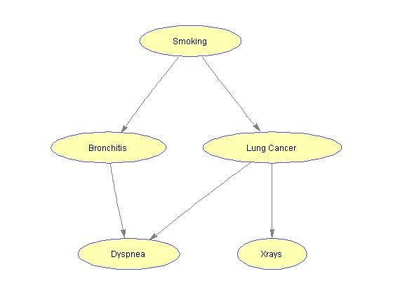
Consider the following example, representing a simplified model to help diagnose the patients arriving at a respiratory clinic. A history of smoking has a direct influence on both whether or not a patient has bronchitis and whether or not a patient has lung cancer. In turn, the presence or absence of lung cancer has direct influence on the results of a chest x-ray test. We are interested in doing probabilistic inference involving features that are not directly related, and for which the conditional probability cannot be readily computed using a simple application of the Bayes' theorem.

Creating the Bayesian Network

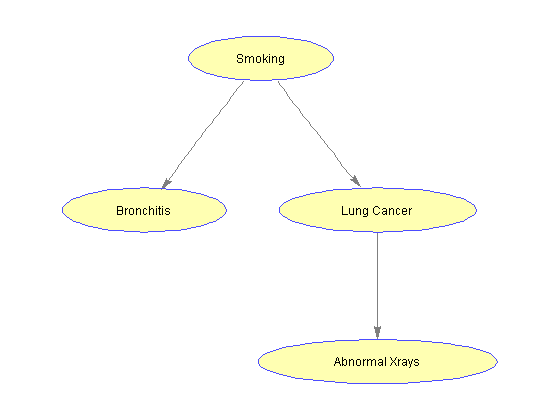
A Bayesian network consists of a direct-acyclic graph (DAG) in which every node represents a variable and every edge represents a dependency between variables. We construct this graph by specifying an adjacency matrix where the element on row i and column j contains the number of edges directed from node i to node j. The variables of the models are specified by the graph's nodes: S (smoking history), B (bronchitis), L (lung cancer) and X (chest x-ray). The variables are discrete and can take only two values: true (t) or false (f).

%=== setup
adj = [0 1 1 0; 0 0 0 0; 0 0 0 1; 0 0 0 0]; % adjacency matrix
nodeNames = {'S', 'B', 'L', 'X'};           % nodes
S = 1; B = 2; L = 3; X = 4;                 % node identifiers
n = numel(nodeNames);                       % number of nodes
t = 1; f  = 2;                              % true and false
values = cell(1,n);                         % values assumed by variables
for i = 1:numel(nodeNames)
    values{i} = [t f];
end

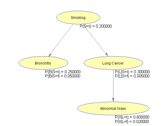
In addition to the graph structure, we need to specify the parameters of the model, namely the conditional probability distribution. For discrete variables, this distribution can be represented as a table (Conditional Probability Table, CPT), which lists the probability that a node takes on each of its value, given the value combinations of its parents.

%=== Conditional Probability Table
CPT{S} = [.2 .8];
CPT{B}(:,t) = [.25 .05] ; CPT{B}(:,f) = 1 - CPT{B}(:,t);
% CPT{L}(:,t) = [.03 .0005]; CPT{L}(:,f) = 1 - CPT{L}(:,t);
CPT{L}(:,t) = [.3 .005]; CPT{L}(:,f) = 1 - CPT{L}(:,t);
CPT{X}(:,t) = [.6 .02]; CPT{X}(:,f) = 1 - CPT{X}(:,t);

Visualizing the Bayesian Network as a Graph

We can visualize the network structure using the biograph object. The properties of nodes and edges can be changed as desidered.

%=== draw the network
nodeLabels = {'Smoking', 'Bronchitis', 'Lung Cancer', 'Abnormal Xrays'};
bg = biograph(adj, nodeLabels, 'arrowsize', 4);
set(bg.Nodes, 'shape', 'ellipse');
bgInViewer = view(bg);

%=== save as figure
bgFig = figure;
copyobj(bgInViewer.hgAxes,bgFig)

%=== annotate using the CPT
[xp, xn] = find(adj);     % xp = parent id, xn = node id
pa(xn) = xp;              % parents
pa(1) = 1;                % root is parent of itself

s1 = cell(1,n); s2 = cell(1,n); pos = zeros(n,2);
for i = 2:n
    pos(i,:) = bgInViewer.Nodes(i).Position;
    s1{i} = sprintf('P(%s|%s=t) = %f', nodeNames{i}, nodeNames{pa(i)}, CPT{i}(1,t));
    s2{i} = sprintf('P(%s|%s=f) = %f', nodeNames{i}, nodeNames{pa(i)}, CPT{i}(2,t));
end

pos(1,:) = bgInViewer.Nodes(1).Position; % root
s1{1} = sprintf('P(%s=t) = %f', nodeNames{1}, CPT{1}(1));
s2{1} = ' ';

text(pos(:,1)+2, pos(:,2)-10, s1)
text(pos(:,1)+2, pos(:,2)-15, s2)

Initializing the Bayesian Network

The process of computing the probability distribution of variables given specific evidence is called probabilistic inference. By exploiting local independencies among nodes, Pearls [1] developed a message-passing algorithm for exact inference in singly-connected networks. The algorithm can compute the conditional probability of any variable given any set of evidence by propagation of beliefs between neighboring nodes. For more information about the message-passing algorithm see [2]. We can create and initiate a Bayesian network for the example under consideration as follows:

root = find(sum(adj,1)==0); % root is any node with no parent
[nodes, edges] = bnMsgPassCreate(adj, values, CPT);
[nodes, edges] = bnMsgPassInitiate(nodes, edges, root)

nodes = 

4x1 struct array with fields:
    id
    values
    parents
    children
    peye
    lambda
    CPT
    P


edges = 

4x4 struct array with fields:
    peyeX
    lambdaX

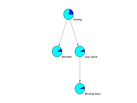
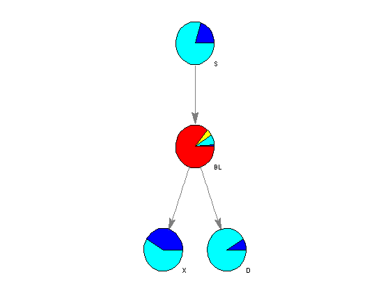
The algorithm parameters, including the conditional probability of each node given the evidence, are stored in the fields of the MATLAB structures nodes and edges. Using the function customnodedraw, we can visualize the distribution of the conditional probability given an empty set of evidence in a series of pie charts, as shown below.

%=== conditional probability given the empty set []
for i = 1:n
    disp(['P(' nodeNames{i}, '|[]) = ' num2str(nodes(i).P(1))]);
end

%=== assign relevant info to each node handle
nodeHandles = bgInViewer.Nodes;
for i = 1:n
    nodeHandles(i).UserData.Distribution = [nodes(i).P];
end

%=== draw customized nodes
bgInViewer.ShowTextInNodes = 'none';

set(nodeHandles, 'shape','circle')
bgInViewer.CustomNodeDrawFcn = @(node) customnodedraw(node);
%bgInViewer.Scale = .7
bgInViewer.dolayout

P(S|[]) = 0.2
P(B|[]) = 0.09
P(L|[]) = 0.064
P(X|[]) = 0.05712

Suppose we are interested in evaluating the likelihood that a patient with bronchitis has lung cancer. We instantiate B=t (true) and we update the network as follows:

%=== inference with B = t
evNode = B;
evValue = t;
[n1, e1, A1, a1] = bnMsgPassUpdate(nodes, edges, [], [], evNode, evValue);

for i = 1:n
    disp(['P(' nodeNames{i}, '|B=t) = ' num2str(n1(i).P(1))]);
end

%== plot and compare
figure(); subplot(2,1,1);
x = cat(1,nodes.P);
bar(x, 'stacked'); set(gca, 'xticklabel', nodeNames);
ylabel('Probability');
title('Initialized network with empty evidence set')
legend({'true', 'false'}, 'location', 'SouthEastOutside')
hold on; subplot(2,1,2);
x1 = cat(1,n1.P);
bar(x1, 'stacked'); set(gca, 'xticklabel', nodeNames);
ylabel('Probability');
title('Updated network with evidence B=true')
legend({'true', 'false'}, 'location', 'SouthEastOutside')

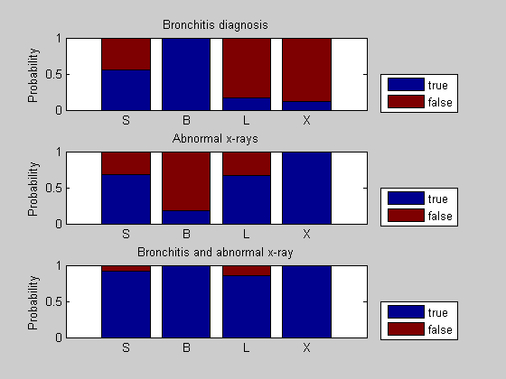
P(S|B=t) = 0.55556
P(B|B=t) = 1
P(L|B=t) = 0.16889
P(X|B=t) = 0.11796

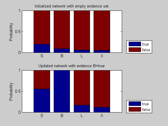
With the observation that the patient has bronchitis (B = t), the probability of a true condition for all other nodes has increased. In particular, the probability of smoking history increases because smoking is one leading cause of chronic bronchitis. In turn, because smoking is also associated with lung cancer, the probability of lung cancer increases and so does the probability of an abnormal chest x-ray test.

Suppose the patient has not been evaluated for bronchitis but the chest x-ray shows some abnormalities. We instantiate X = t and we intialize again the network with the new evidence.

evNode = X;
evValue = t;
[n2, e2, A2, a2] = bnMsgPassUpdate(nodes, edges, [], [], evNode, evValue);

for i = 1:n
    disp(['P(' nodeNames{i}, '|X=t) = ' num2str(n2(i).P(1))]);
end

P(S|X=t) = 0.67927
P(B|X=t) = 0.18585
P(L|X=t) = 0.67227
P(X|X=t) = 1

Given the observed abnormal x-ray results, the probability of lung cancer has increased significantly because of the direct dependency of node X (x-rays) on node L (lung cancer).

Finally, suppose the patient has both been diagnosed with bronchitis and received positive results for his/her chest x-ray. We update the previous state of the network (X = t) with the new evidence(B = t), as shown below:

evNode = B;
evValue = t;
[n3, e3, A3, a3] = bnMsgPassUpdate(n2, e2, A2, a2, evNode, evValue);

for i = 1:n
    disp(['P(' nodeNames{i}, '|B=t,X=t) = ' num2str(n3(i).P(1))]);
end

P(S|B=t,X=t) = 0.91372
P(B|B=t,X=t) = 1
P(L|B=t,X=t) = 0.85908
P(X|B=t,X=t) = 1

We can compare the three situations by plotting the probabilities as bar charts. Evidence of bronchitis and evidence of abnormal x-rays increase the probability of lung cancer and smoking history, one indirectly and the other directly.

figure(); subplot(3,1,1);
bar(x1,  'stacked'); set(gca, 'xticklabel', nodeNames);
ylabel('Probability'); title('Bronchitis diagnosis');
legend({'true', 'false'}, 'location', 'SouthEastOutside')
hold on; subplot(3,1,2);
x2 = cat(1,n2.P);
bar(x2,'stacked'); set(gca, 'xticklabel', nodeNames);
ylabel('Probability'); title('Abnormal x-rays');
legend({'true', 'false'}, 'location', 'SouthEastOutside')
hold on; subplot(3,1,3);
x3 = cat(1,n3.P);
bar(x3, 'stacked'); set(gca, 'xticklabel', nodeNames);
ylabel('Probability'); title('Bronchitis and abnormal x-ray');
legend({'true', 'false'}, 'location', 'SouthEastOutside')

We can now compare the effect of a positive versus negative bronchitis diagnosis in presence of abnormal x-ray results. We instantiate B = f (false) and compare with previous estimates B = t (true).

evNode = B;
evValue = f;
[n4, e4, A4, a4] = bnMsgPassUpdate(n2, e2, [], [], evNode, evValue);

for i = 1:n
    disp(['P(' nodeNames{i}, '|B=f,X=t) = ' num2str(n4(i).P(1))]);
end

figure();
bar3([n3(S).P(:,t) n4(S).P(:,t); n3(L).P(:,t) n4(L).P(:,t)]);
colormap(summer); zlabel('Probability');
set(gca,'xticklabel',{'Smoking','Lung Cancer'},'yticklabel', {'With Bronchitis', 'Without Bronchitis'});
set(gca,'xticklabel',{'With Bronchitis','Without Bronchitis'},'yticklabel', {'Smoking','Lung Cancer'});
title('Conditional probabilities with evidence of abnormal x-ray results')
view(50,35);

P(S|B=f,X=t) = 0.62575
P(B|B=f,X=t) = 0
P(L|B=f,X=t) = 0.62962
P(X|B=f,X=t) = 1

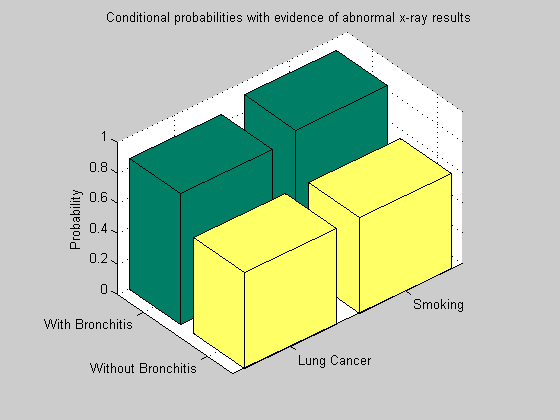
When bronchitis is ruled out (B = f), the probability of smoking history decreases with respect to the case in which the bronchitis is confirmed (B = t). The effect is propagated across the network and affects the probability of lung cancer in a similar manner.

Expanding the Network

Among various symptoms related to lung cancer and bronchitis is shortness of breath (dyspnea). We want to model the relationship of this condition within the considered Bayesian Network. We introduce a node D and modify the adjacency matrix accordingly.

%=== add node D to the network
D = 5;
CPT{D}(:,:,t) = [.75 .1; .5 .05];
CPT{D}(:,:,f) = 1 - CPT{D}(:,:,t);
values{D} =  [1 2];
adj(end+1,:) = [0 0 0 0];
adj(:,end+1) = [0 1 1 0 0];

%=== draw the updated network
nodeLabels = {'Smoking', 'Bronchitis', 'Lung Cancer', 'Xrays', 'Dyspnea'};
nodeSymbols = {'S', 'B', 'L', 'X', 'D'};
bg = biograph(adj, nodeLabels, 'arrowsize', 4);
nodeHandles= bg.Nodes;
set(nodeHandles, 'shape', 'ellipse');
view(bg)

With the introduction of node D, the network is not singly-connected anymore. In fact, there are more than one chain between any two nodes (i.e., S and D). We can check this property by considering the undirected graph associated with the network and veryfying that it is not acyclic.

isAcyclic = graphisdag(sparse(adj | adj'))

isAcyclic =

     0

In order to use the algorithm for exact inference described above, we must transform the new, multiply-connected network into a singly-connected network. Several approaches can be used, including clustering of parent nodes (in our case B and L) into a single node as follows.

First, we combine the adjacency matrix entries corresponding to the nodes B and L into one entry associated to node BL. The node BL can take up to four values, corresponding to all possible combinations of values of the original nodes B and L. Then, we update the conditional probability distribution considering that B and L are conditionally independent given the node S, that is P(BL|S) = P(B,L|S) = P(B|S) * P(L|S).

%=== combine B and L
adj(B,:) = adj(B,:) | adj(L,:);
adj(:,B) = adj(:,B) | adj(:,L);
adj(L,:) = []; adj(:,L) = [];

%=== update the probability distribution accordingly
b1 = kron(CPT{B}(1,:), CPT{L}(1,:));
b2 = kron(CPT{B}(2,:), CPT{L}(2,:));
x = [CPT{X}(1,:) CPT{X}(1,:)];
d =  reshape((CPT{D}(:,:,1))', 1, 4);

%=== update the node values
S = 1; BL = 2; X = 3; D = 4;
nodeNames = {'S', 'BL', 'X', 'D'};
tt = 1; tf = 2; ft = 3; ff = 4;
values{BL} = 1:4;
values(L) = [];

%=== create a clustered Conditional Probability Table
cCPT{S} = CPT{S};
cCPT{BL}(t,:) = b1; cCPT{BL}(f,:) = b2;
cCPT{D}(:,t) = d; cCPT{D}(:,f) = 1 - d;
cCPT{X}(:,t) = x; cCPT{X}(:,f) = 1 - x;

%=== create and intiate the net
root = find(sum(adj,1)==0); % root (node with no parent)
[cNodes, cEdges] = bnMsgPassCreate(adj, values, cCPT);
[cNodes, cEdges] = bnMsgPassInitiate(cNodes, cEdges, root);

for i = 1:n
    disp(['P(' nodeNames{i}, '|[]) = ' num2str(cNodes(i).P(1))]);
end

P(S|[]) = 0.2
P(BL|[]) = 0.0152
P(X|[]) = 0.4128
P(D|[]) = 0.08634

Drawing the Expanded Network

%=== draw the network
nodeLabels = {'Smoking', 'Bronchitis or Lung Cancer', 'Abnormal X-rays', 'Dyspnea'};
cbg = biograph(adj, nodeNames, 'arrowsize', 4);
set(cbg.Nodes, 'shape', 'ellipse');
cbgInViewer = view(cbg);

%=== assign relevant info to each node handle
cnodeHandles = cbgInViewer.Nodes;
for i = 1:n
    cnodeHandles(i).UserData.Distribution = [cNodes(i).P];
end

%=== draw customized nodes
set(cnodeHandles, 'shape','circle')
colormap(summer)
cbgInViewer.ShowTextInNodes = 'none';
cbgInViewer.CustomNodeDrawFcn = @(node) customnodedraw(node);
cbgInViewer.Scale = .7
cbgInViewer.dolayout

Biograph object with 4 nodes and 3 edges.

Performing Exact Inference on Clustered Trees

Suppose a patient complains of dyspnea (D=t). We would like to evaluate the likelihood that this symptom is related to either lung cancer or bronchitis.

[n5, e5, A5, a5] = bnMsgPassUpdate(cNodes, cEdges, [], [], D, t);

Because node B and node L are clustered into the node BL, we have to calculate their individual conditional probabilities by considering the appropriate value combinations. The conditional probabilities in BL correspond to the following B and L value combinations: BL = tt if B = t and L = t; BL = tf if B = t and L = f; BL = ft if B = f and L = t; BL = ff if B = f and L = f. Therefore P(B|evidence) is equal to the sum of the first two elements of P(BL|evidence), and similarly, P(L|evidence) is equal to the sum of the first and third elements in P(BL|evidence).

p(1,:) = n5(S).P;
p(2,:) = [sum(n5(BL).P([tt,tf])), 1-sum(n5(BL).P([tt,tf]))];     % P(B|evidence)
p(3,:) = [sum(n5(BL).P([tt,ft])), 1-sum(n5(BL).P([tt,ft]))]; % P(L|evidence)
p(4,:) = n5(X).P;
p(5,:) = n5(D).P;

for i = 1:5
    disp(['P(' nodeSymbols{i}, '|D=t) = ' num2str(p(i,1))]);
end

P(S|D=t) = 0.49224
P(B|D=t) = 0.21867
P(L|D=t) = 0.41464
P(X|D=t) = 0.48293
P(D|D=t) = 1

When dyspnea is present, both the likelihood of bronchitis and lung cancer increase. This makes sense, since both illnesses have dyspnea as symptom and the patient is indeed exhibiting this symptom.

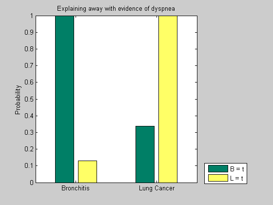
Explaining Away the Lung Cancer

As we can see in the graph, the dyspnea symptom has dependency both on bronchitis and lung cancer. Consider the effect of a bronchitis diagnosis on the likelihood of lung cancer.

%=== adjust the CPT to reflect B = 1 before clustering into BL node
B = 2; L = 3;
CPT{B}(:,1) = [1 1] ; CPT{B}(:,2) = 1 - CPT{B}(:,1);
b1 = kron(CPT{B}(1,:), CPT{L}(1,:));
b2 = kron(CPT{B}(2,:), CPT{L}(2,:));

%=== create a clustered Conditional Probability Table
BL = 2;
cCPT{BL}(1,:) = b1; cCPT{BL}(2,:) = b2;

%=== create and intiate the net
root = find(sum(adj,1)==0); % root (node with no parent)
[cNodes, cEdges] = bnMsgPassCreate(adj, values, cCPT);
[cNodes, cEdges] = bnMsgPassInitiate(cNodes, cEdges, root);

%=== instantiate for F = 1
[n7, e7, A7, a7] = bnMsgPassUpdate(cNodes, cEdges, [], [], D, t);
w(1,:) = n7(S).P;
w(2,:) = [sum(n7(BL).P([tt,tf])), 1-sum(n7(BL).P([tt,tf]))];     % P(B|evidence)
w(3,:) = [sum(n7(BL).P([tt,ft])), 1-sum(n7(BL).P([tt,ft]))]; % P(L|evidence)
w(4,:) = n7(X).P;
w(5,:) = n7(D).P;

for i = 1:5
    disp(['P(' nodeSymbols{i}, '|B=t,D=t) = ' num2str(w(i,1))]);
end

P(S|B=t,D=t) = 0.41667
P(B|B=t,D=t) = 1
P(L|B=t,D=t) = 0.33898
P(X|B=t,D=t) = 0.4678
P(D|B=t,D=t) = 1

When a patient complains of dyspnea and is diagnosed with bronchitis, the conditional probability of lung cancer is lower.

Consider now the effect of a lung cancer diagnosis on the likellihood of bronchitis.

%=== adjust the CPT to reflect L = 1 before clustering into BL node
B = 2; L = 3;
CPT{B}(:,t) = [.25 .05] ; CPT{B}(:,f) = 1 - CPT{B}(:,t);
CPT{L}(:,t) = [1 1]; CPT{L}(:,f) = 1 - CPT{L}(:,t);

b1 = kron(CPT{B}(t,:), CPT{L}(t,:));
b2 = kron(CPT{B}(f,:), CPT{L}(f,:));

BL = 2;
cCPT{BL}(t,:) = b1; cCPT{BL}(f,:) = b2;

%=== create and intiate the net
root = find(sum(adj,1)==0); % root (node with no parent)
[cNodes, cEdges] = bnMsgPassCreate(adj, values, cCPT);
[cNodes, cEdges] = bnMsgPassInitiate(cNodes, cEdges, root);

%=== instantiate for D = 1
[n8, e8, A8, a8] = bnMsgPassUpdate(cNodes, cEdges, [], [], D, t);
v(1,:) = n8(S).P;
v(2,:) = [sum(n8(BL).P([tt,tf])), 1-sum(n8(BL).P([tt,tf]))];     % P(B|evidence)
v(3,:) = [sum(n8(BL).P([tt,ft])), 1-sum(n8(BL).P([tt,ft]))]; % P(L|evidence)
v(4,:) = n8(X).P;
v(5,:) = n8(D).P;

for i = 1:5
    disp(['P(' nodeSymbols{i}, '|L=t,D=t) = ' num2str(v(i,1))]);
end

P(S|L=t,D=t) = 0.21531
P(B|L=t,D=t) = 0.12919
P(L|L=t,D=t) = 1
P(X|L=t,D=t) = 0.6
P(D|L=t,D=t) = 1

If a patient is diagnosed with lung cancer in presence of dyspnea, the likelihood of bronchitis decreases significantly. This phenomenon is called "explaining away" and refers to the situations in which the chances of one cause decrease significantly when the chances of the competing cause increase.

We can observe the "explaining away" phenomenon in the two situations described above by comparing the conditional probabilities of node L and B in the two cases. When the evidence for B is high, the likelihood of L is relatively low, and viceversa, when the evidence for L is high, the likelihood of B is low.

y = [w(2:3,1)  v(2:3,1)];
figure();
bar(y);
set(gca, 'xticklabel', {'Bronchitis', 'Lung Cancer'});
ylabel('Probability'); title('Explaining away with evidence of dyspnea')
legend('B = t', 'L = t', 'location', 'SouthEastOutside');
colormap(summer)

References

[1] Pearl J., "Probabilistic Reasoning in Intelligent Systems", Morgan Kaufmann, San Mateo, California, 1988.

[2] Neapolitan R., "Learning Bayesian Networks", Pearson Prentice Hall, Upper Saddle River, New Jersey, 2004.